merge_samples

merge_samples can be very useful if you’d like to see what happens to an analysis if you remove the indivual effects between replicates or between samples from a particular explanatory variable. With the merge_samples function, the abundance values of merged samples are summed, so make sure to do any preprocessing to account for differences in sequencing effort before merging or you will achieve a sequencing-effort-weighted average (which you may want, but keep in mind).

Let’s first remove unobserved OTUs (sum 0 across all samples), and add a human-associated variable with which to organize data later in the plots.

library("phyloseq"); packageVersion("phyloseq")

## [1] '1.22.3'

Load data, remove empty samples, add a new sample_data variable to the dataset.

data(GlobalPatterns)
GP = GlobalPatterns
GP = prune_taxa(taxa_sums(GlobalPatterns) > 0, GlobalPatterns)
humantypes = c("Feces", "Mock", "Skin", "Tongue")
sample_data(GP)$human <- get_variable(GP, "SampleType") %in% humantypes

Now on to the merging examples

mergedGP = merge_samples(GP, "SampleType")
SD = merge_samples(sample_data(GP), "SampleType")
print(SD[, "SampleType"])

##                    SampleType
## Feces                       1
## Freshwater                  2
## Freshwater (creek)          3
## Mock                        4
## Ocean                       5
## Sediment (estuary)          6
## Skin                        7
## Soil                        8
## Tongue                      9

print(mergedGP)

## phyloseq-class experiment-level object
## otu_table()   OTU Table:         [ 18988 taxa and 9 samples ]
## sample_data() Sample Data:       [ 9 samples by 8 sample variables ]
## tax_table()   Taxonomy Table:    [ 18988 taxa by 7 taxonomic ranks ]
## phy_tree()    Phylogenetic Tree: [ 18988 tips and 18987 internal nodes ]

sample_names(GP)

##  [1] "CL3"      "CC1"      "SV1"      "M31Fcsw"  "M11Fcsw"  "M31Plmr" 
##  [7] "M11Plmr"  "F21Plmr"  "M31Tong"  "M11Tong"  "LMEpi24M" "SLEpi20M"
## [13] "AQC1cm"   "AQC4cm"   "AQC7cm"   "NP2"      "NP3"      "NP5"     
## [19] "TRRsed1"  "TRRsed2"  "TRRsed3"  "TS28"     "TS29"     "Even1"   
## [25] "Even2"    "Even3"

sample_names(mergedGP)

## [1] "Feces"              "Freshwater"         "Freshwater (creek)"
## [4] "Mock"               "Ocean"              "Sediment (estuary)"
## [7] "Skin"               "Soil"               "Tongue"

identical(SD, sample_data(mergedGP))

## [1] TRUE

As emphasized earlier, the OTU abundances of merged samples are summed. Let’s investigate this ourselves looking at just the top10 most abundance OTUs.

OTUnames10 = names(sort(taxa_sums(GP), TRUE)[1:10])
GP10  = prune_taxa(OTUnames10,  GP)
mGP10 = prune_taxa(OTUnames10, mergedGP)
ocean_samples = sample_names(subset(sample_data(GP), SampleType=="Ocean"))
print(ocean_samples)

## [1] "NP2" "NP3" "NP5"

otu_table(GP10)[, ocean_samples]

## OTU Table:          [10 taxa and 3 samples]
##                      taxa are rows
##         NP2   NP3   NP5
## 329744   91   126   120
## 317182 3148 12370 63084
## 549656 5045 10713  1784
## 279599  113   114   126
## 360229   16    83   786
## 94166    49   128   709
## 550960   11    86    65
## 158660   13    39    28
## 331820   24   101   105
## 189047    4    33    29

rowSums(otu_table(GP10)[, ocean_samples])

## 329744 317182 549656 279599 360229  94166 550960 158660 331820 189047 
##    337  78602  17542    353    885    886    162     80    230     66

otu_table(mGP10)["Ocean", ]

## OTU Table:          [10 taxa and 1 samples]
##                      taxa are columns
##       329744 317182 549656 279599 360229 94166 550960 158660 331820 189047
## Ocean    337  78602  17542    353    885   886    162     80    230     66

Let’s look at the merge graphically between two richness estimate summary plots. Note that we are ignoring our own advice and not-performing any preprocessing before this merge. Since these are richness estimates we are probably safe.

plot_richness(GP, "human", "SampleType", title="unmerged")

## Warning: Removed 130 rows containing missing values (geom_errorbar).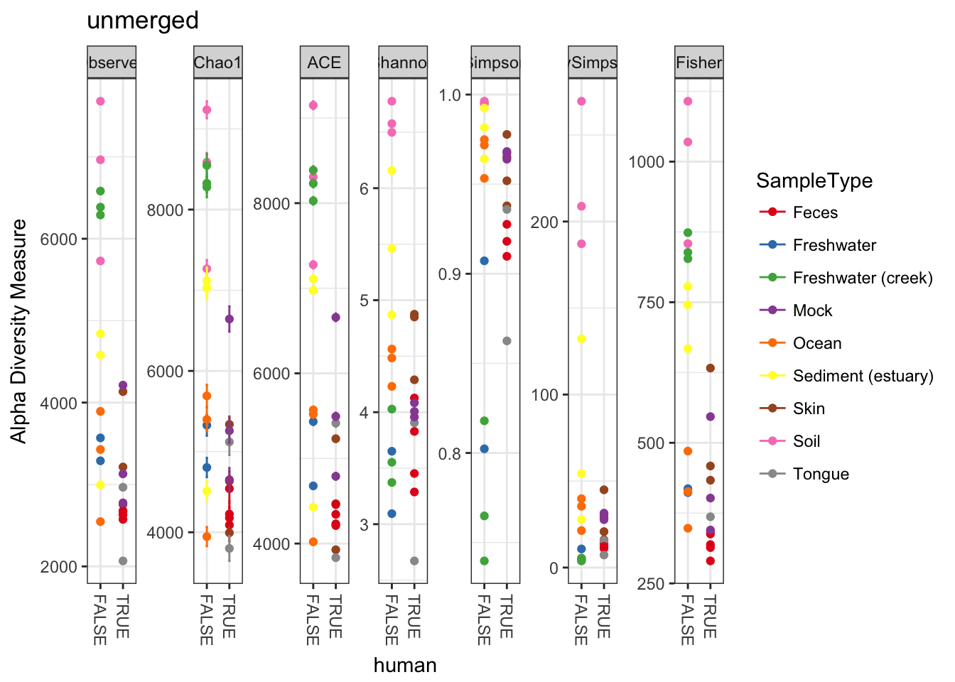

The merge can do some weird things to sample variables. Let’s re-add these variables to the sample_data before we plot.

sample_data(mergedGP)$SampleType = sample_names(mergedGP)
sample_data(mergedGP)$human = sample_names(mergedGP) %in% humantypes
plot_richness(mergedGP, "human", "SampleType", title="merged")

## Warning: Removed 45 rows containing missing values (geom_errorbar).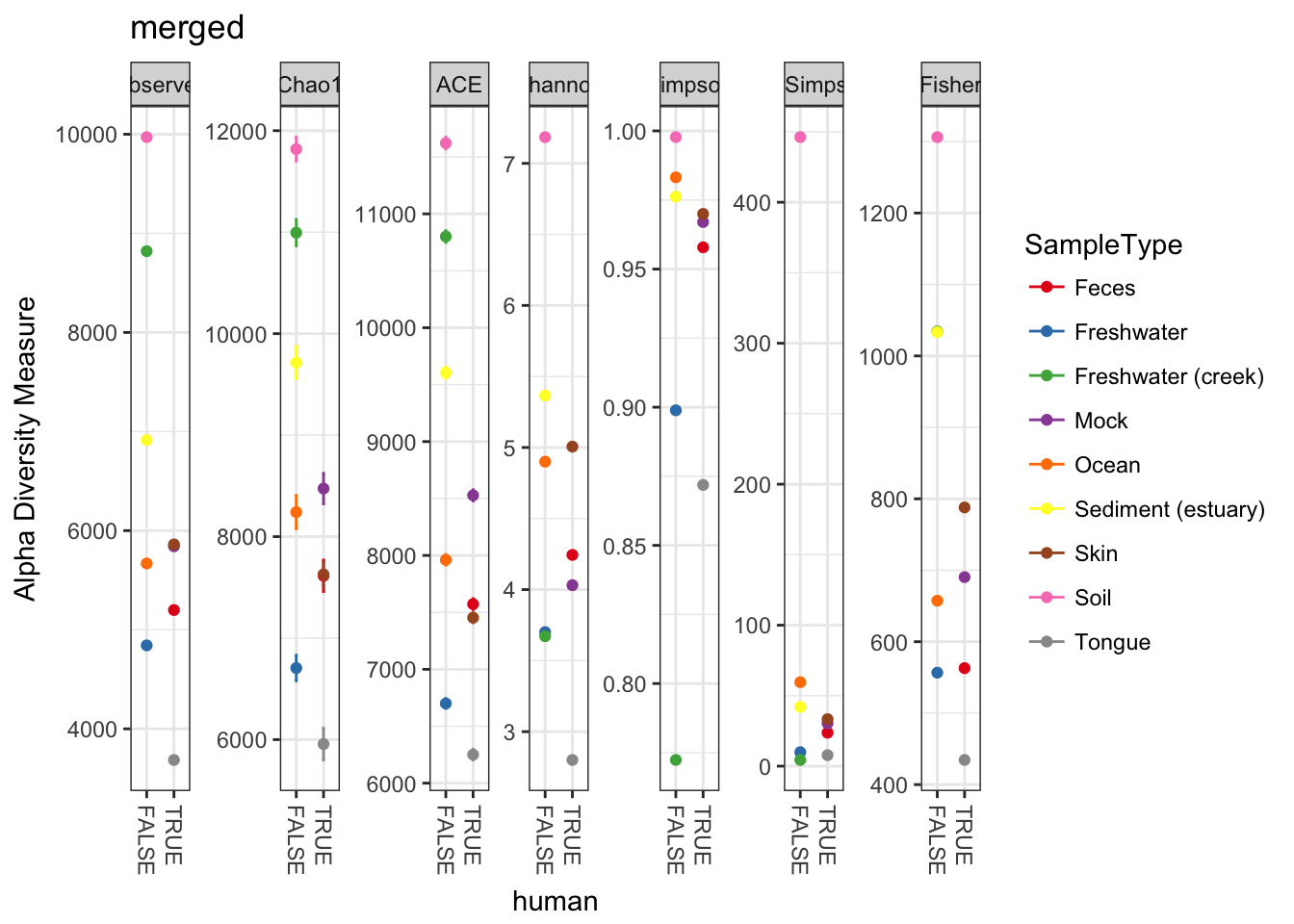

Perhaps not surprisingly, when we combine the abundances of non-replicate samples from the same environment, the estimates of absolute richness increase for each environment. More to the example, however, the new merged plot is easier to read and interpret, which is one of the reasons one might use the merge_samples function.

merge_taxa

One of the sources of “noise” in a microbial census dataset is a fine-scaled definition for OTU that blurs a pattern that might be otherwise evident were we to consider a higher taxonomic rank. The best way to deal with this is to use the agglomeration functions tip_glom or tax_glom that merge similar OTUs based on a phylogenetic or taxonomic threshold, respectively. However, for either function to work, it must be capable of merging two or more OTUs that have been deemed “equivalent”.

The following is an example of merge_taxa in action, using a tree graphic to display the before and after of the merge, and also show how the merge affects not just the OTU table, but all data components with OTU indices.

We will use an example dataset that was previously imported into phyloseq with the variable name closedps and saved within an RData binary file, "example-data.RData".

load("example-data.RData")
plot_tree(closedps, color="Treatment", size="abundance", sizebase=2, label.tips="taxa_names")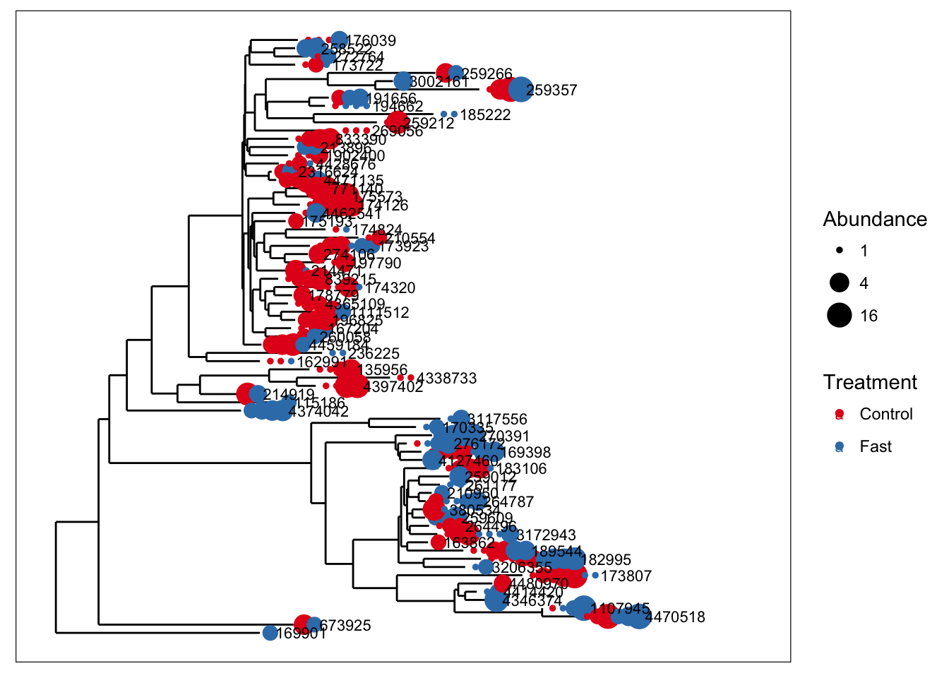

Now let’s use merge_taxa to merge the first 8 OTUS of closedps into one new OTU. By choosing 2 as the optional third argument to merge_taxa, we are combining the counts of these 8 OTUs into the index for the second OTU. The default is to use the first OTU of the second argument.

x1 = merge_taxa(closedps, taxa_names(closedps)[3:27], 2)
plot_tree(x1, color="Treatment", size="abundance", sizebase=2, label.tips="taxa_names")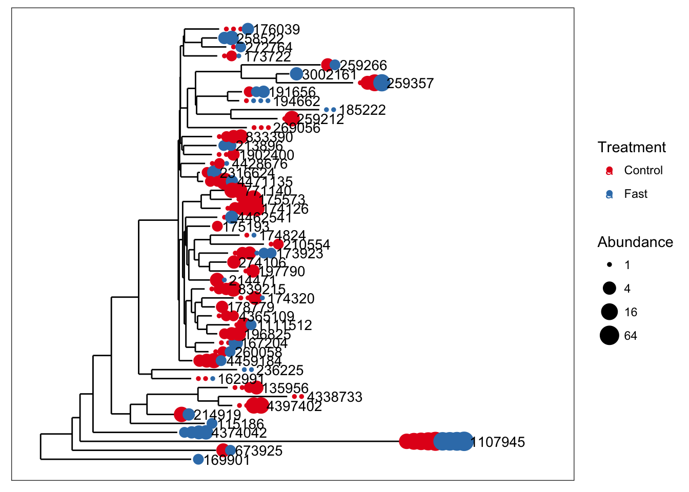

merge_phyloseq

As said earlier, merge_phyloseq is a convenience/support tool to help get your data into the right format. Here is an example in which we extract components from an example dataset, and then build them back up to the original form using merge_phyloseq along the way.

Let’s split apart the “Global Patterns” example dataset into some components

data(GlobalPatterns)
tree = phy_tree(GlobalPatterns)
tax  = tax_table(GlobalPatterns)
otu  = otu_table(GlobalPatterns)
sam  = sample_data(GlobalPatterns)
otutax = phyloseq(otu, tax)
otutax

## phyloseq-class experiment-level object
## otu_table()   OTU Table:         [ 19216 taxa and 26 samples ]
## tax_table()   Taxonomy Table:    [ 19216 taxa by 7 taxonomic ranks ]

As you can see, our new otutax object has just the OTU table and taxonomy table. Now let’s use merge_phyloseq to build up the original GlobalPatterns object, and compare to make sure they are identical. Note how the arguments to merge_phyloseq are a mixture of multi-component (otutax) and single component objects.

GP2 = merge_phyloseq(otutax, sam, tree)
identical(GP2, GlobalPatterns)

## [1] TRUE

otusamtree = phyloseq(otu, sam, tree)
GP3 = merge_phyloseq(otusamtree, otutax)
GP3

## phyloseq-class experiment-level object
## otu_table()   OTU Table:         [ 19216 taxa and 26 samples ]
## sample_data() Sample Data:       [ 26 samples by 7 sample variables ]
## tax_table()   Taxonomy Table:    [ 19216 taxa by 7 taxonomic ranks ]
## phy_tree()    Phylogenetic Tree: [ 19216 tips and 19215 internal nodes ]

identical(GP3, GlobalPatterns)

## [1] FALSE

GP4 = merge_phyloseq(otusamtree, tax_table(otutax))
GP4

## phyloseq-class experiment-level object
## otu_table()   OTU Table:         [ 19216 taxa and 26 samples ]
## sample_data() Sample Data:       [ 26 samples by 7 sample variables ]
## tax_table()   Taxonomy Table:    [ 19216 taxa by 7 taxonomic ranks ]
## phy_tree()    Phylogenetic Tree: [ 19216 tips and 19215 internal nodes ]

identical(GP4, GlobalPatterns)

## [1] TRUE